Over the years several modeling styles have been developed but often it is unclear what are the differences between them. In this joint post, we, (
Yang Zhou and myself) would like to compare and contrast four modeling approaches widely used in Computational Social Science, namely: System Dynamics (SD) models, Agent-based Models (ABM), Cellular Automata (CA) models, and Discrete Event Simulation (DES). For a review of their undying mechanisms and core components of each readers are referred to Gilbert and Troitzsch’s (2005) “
Simulation for the Social Scientist“
To compare and contrast the differences in how these models work and how their underlying mechanisms generate outputs, we needed a common problem to test them against with the same set of model parameters. While one could choose a more complex example, here we decided to chose one of the simplest models we know. Specifically, we chose to model the spread of a disease specifically using a Susceptible-Infected-Recovered (SIR) epidemic model. Our inspiration for this came from the SD model outlined in the great book “
Introduction to Computational Science: Modeling and Simulation for the Sciences” by Shiflet and Shiflet (2014) which was implemented in NetLogo from the accompanying
website. For the remaining models (i.e. the ABM, CA, and DES) we created models from scratch in
NetLogo. Below we will introduce how we built each model, before showing the results from the four models with the same set of parameters, which allows us to compare the results of the models. The source code, further documentation for the four models can be found over at
Yang Zhou’s website and
GitHub page.
The System Dynamics Model
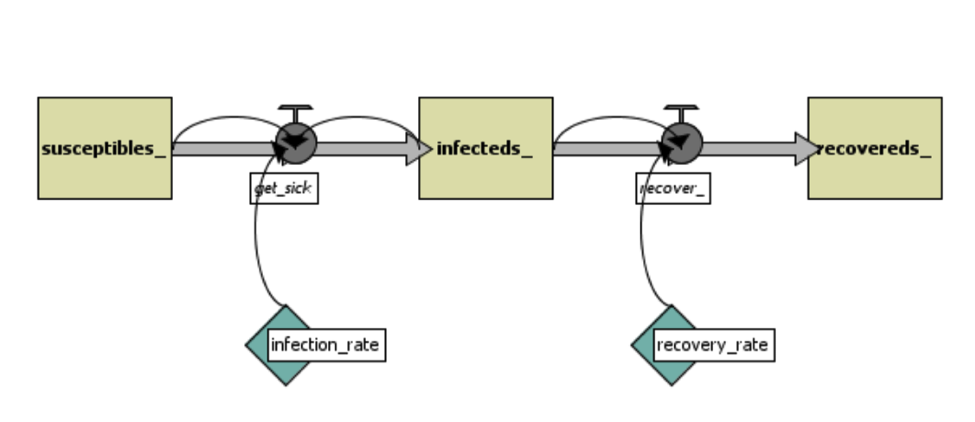
In the system dynamics model from Shiflet and Shiflet (2014), one person is infected at start. Infected people can infect susceptible people. The population of infected will always increase by (number of infected * number of susceptible * InfectionRate * change in time dt). The infected people may recover. The amount of people that will recover in an iteration is always equal to (number of infected * RecoveryRate * change in time dt). Figure 1 illustrates the system dynamics process while Figure 2 shows the SIR process as a flowchart.
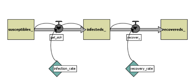 |
| Figure 1. System Dynamics process (source: Shiflet and Shiflet, 2014) |
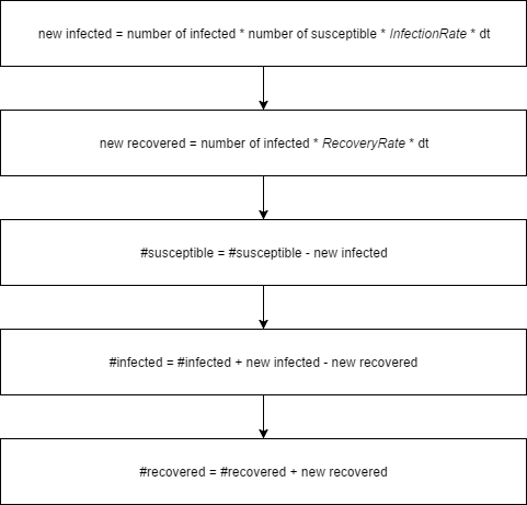 |
| Figure 2. System Dynamics flowchart |
The Agent-based Model
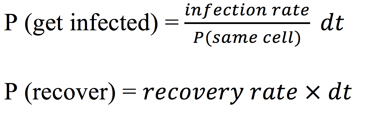
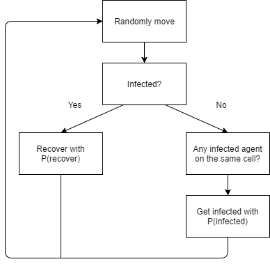
As in the case for the SD model, at the beginning of the simulation, one agent is infected. Agents are randomly distributed on the landscape, and in the beginning of each iteration, they turn to a random direction and move forward by one cell. During each iteration, an infected agent may infect other agents on the same cell. This is different from how the SD model works, specifically the probability of getting infected. In the SD model, the infection rate is the infection rate on the entire population. In the ABM, the probability of becoming infected is equal to the infection rate divided by the probability of an agent to be in the same cell, multiplied by the change in time. Each infected agent has a probability to recover in each time period, which equals to the recovery rate times the change in time. The equations in the ABM are the following:
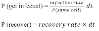
Where P(same cell) = probability to be on the same cell, equals 1 divided by total number of cells; dt = change in time. Figure 3 illustrates the agent decision process while Figure 4 shows the display of the ABM
 |
| Figure 3. Agent-based Modeling: agent decision process |
|
|
|
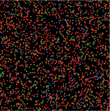 |
| Figure 4. Display of the ABM. Green = susceptible. Red = infected. Blue = recovered. |
The Cellular Automata Model
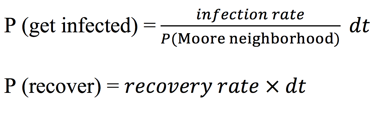
At the beginning of the simulation, one cell is infected. During each iteration (dt), the infected cell can infect other cells in its Moore neighborhood (i.e. 8 surrounding cells). The landscape will be a n by n square, and n is equal to the square root of the number of people to be created at the beginning of the simulation. Wrapping is enabled both horizontally and vertically. Similar to the ABM, we would like to map the probability of becoming infected to the one in the SD model. In the CA model, the probability of becoming infected is equal to the infection rate divided by the probability to be in the Moore neighborhood, multiplied by the change in time. Each infected cell has a probability to recover in each time period, which is based on the recovery rate multiplied by the change in time. The equations here are:
Figure 5 shows the changing process of the cells while Figure 6 shows the display of the CA model.
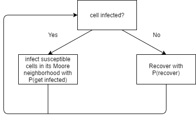 |
| Figure 5. Cellular Automata cell changing process |
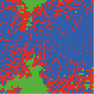 |
| Figure 6. Display of the CA model. Green = susceptible. Red = infected. Blue = recovered. |
The Discrete Event Simulation Model
In a Discrete Event Simulation model (aka. queuing model), there are three abstract types of objects: 1) servers, 2) customers, 3) queues, which is quite different from the CA and ABMs.
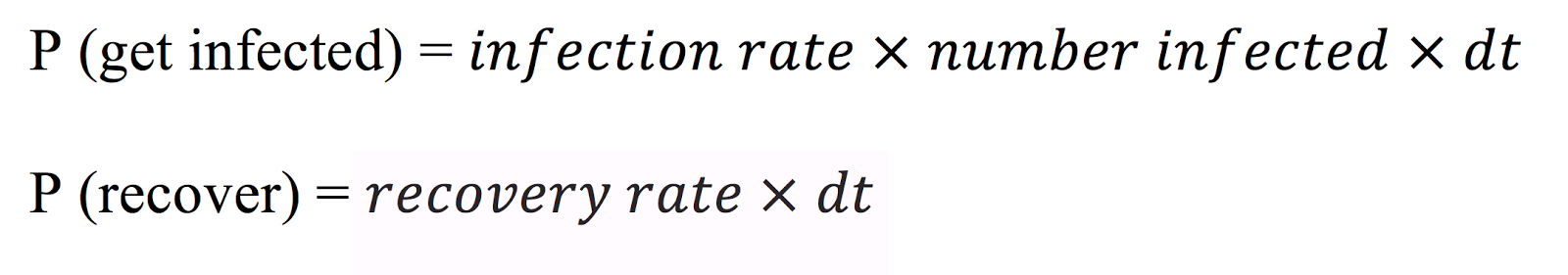
So to implement a SIR model as a DES Servers are the processes of becoming infected and recovering. The durations people stay with the servers represent the process of becoming infected and becoming recovered. Customers are susceptible people to be infected, and infected people are waiting to recover. We assume there are two queues in this model. As susceptible objects (i.e. individuals) are created, queues for infection are formed while people are waiting to be infected. On the other hand, as people get infected, they form a second queue waiting to recover. During each iteration (dt), each object in queue has a probability to get become infected. Each infected agent object has a probability to recover which is equal to RecoveryRate. After agents recover, they enter the sink of recovered people. The equations can be written as follow:
While the whole process is illustrated in Figure 7.
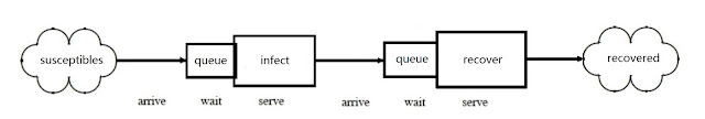 |
| Figure 7. Discrete Event Simulation process. |
Results from the Implementations
Now that the models have been briefly described. We turn to how using the same set of parameters lead to different results. The default parameters being used in each model are: number of susceptible people at setup = 2500, Infection Rate = 0.002, Recovery Rate = 0.5, change of time (dt) = 0.001, and the numbers of people in each status are recorded. Since the SD model has no randomness and will always give the same result, it is run only once. Each of the other three models were run for 10 times (feel free to run them more if you wish), and then we took the average of the ten results and show them in Figure 8. The stop condition is that no individual left to be infected.
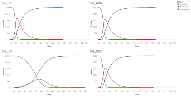 |
| Figure 8. Results for the different models. Clockwise from top left: SD model, ABM, DES and CA |
In the four models, we observe the same pattern: the number of susceptible people decreases, the number of infected people increases first and then decrease again, and the number of recovered people increase over time. However, each model realization also shows a lot of differences in how such patterns play out.
First of all, the SD model has the smallest number of iterations before no one is infected. The number of iterations shown on the graph are the average of the ten runs, since the runs range from smaller to larger numbers (except for the SD model, which only has one run). The SD model only took 17451 iterations to stop, while the ABM took 19145 iterations (on average), the DES model took 18645 iterations (on average). The CA model took the longest time on average for no more individuals to be infected, it took 25680 iterations (on average).
The results of the SD, ABM and DES models while appearing to be very similar to each other. In the sense, that the number of infected people increase fast at first and reaches a peak number of over 1500 at more than 2000 iterations (2272 for SD, 2403 for ABM, 2538 for DES). On the other hand, in the CA model, the number of infected people increases much slower due to the diffusion mechanism of the CA model and never reaches an amount as high as in the former models.
An important characteristic of the SD model is that there is no randomness in the model, so no matter how many times you run this model, you will get the same result. In the other three models, getting infected or recover always depend on a probability function, so there is difference in every run.
Furthermore, people in the SD model and the DES model are homogeneous, and everyone has the same probability to becoming infected or recovering from an infection, although these rates change over time, they do not vary among the different people in the population. On the other hand, in the ABM and the CA model, people (represented by moving agents or static cells) are heterogenous in the sense that they have different locations. Only susceptible people around an infected individual can be infected. It is interesting that when people can move around, like in the ABM, the result is similar to the SD model, though the ABM takes a little more time to recover (19145 iterations in ABM vs. 17451 iterations in SD). When people are static and the number of people on the same space is limited (one cell in one space in this case), like in the CA model, the infection process becomes slower and it takes longer for everyone to recover.
To test how the models are sensitive to a specific parameter we now present what happens if we increase the infection rate in each model from 0.002 to 0.02 and show the results shown in Figure 9. As to be expected as the infection rate increased, the number of susceptible people decrease at a much faster rate. However, the SD, the ABM, and the DES models are still similar to each other, while the infection in the CA model is slower. The average number of iterations for these models are: 15807 (SD), 15252 (ABM), 16937 (CA), 16677 (DES). By increasing the infection rate the total number of iterations of each model has decreased, with the CA model still taking the longest time to converge. The peak of infected people in each model are on average: 2363 people at 255 iterations (SD), 2310 people at 363 iterations (ABM), 2035 people at 1019 iterations (CA), 2340 people at 286 iterations (DES). The CA model takes a longer time and reaches a lower peak.
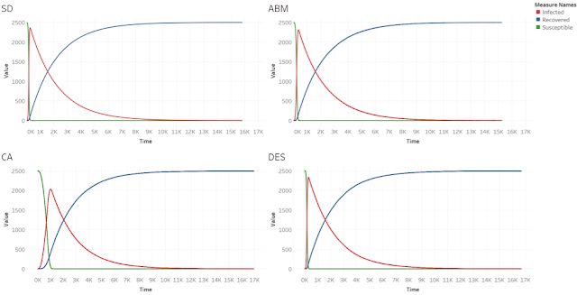 |
| Figure 9. Results for the different models with infection rate = 0.02. Clockwise from top left: SD model, ABM, DES and CA. |
These models are only simple examples of how a SIR model can be implemented in different modeling techniques, but in reality, if we were to model disease propagation in more detail we would need to consider many other things such as people could be both moving through space (i.e. traveling to work) and static (i.e. staying at home), and the capacity of each cell is always limited to some amount.
References:
Gilbert, N. and Troitzsch, K.G. (2005), Simulation for the Social Scientist (2nd Edition), Open University Press, Milton Keynes, UK.
Shiflet, A.B. and Shiflet, G.W. (2014), Introduction to Computational Science: Modeling and Simulation for the Sciences (2nd Edition), Princeton University Press, Princeton, NJ.
More information about the models and to download them please visit Yang Zhou’s website.
Continue reading »